This course covers three core aspects of robotics: perception, planning, and learning. These are highly relevant to modern academic research and industrial applications of robotics. The course is primarily taught by Dr. Pratik Chaudhari, who also:
- advised my senior capstone project
- served as the instructor in my other favorite course at Penn
- advised my graduate studies
State Estimation
"The state of a robot is a set of quantities, such as position, orientation, and velocity, that, if known, fully describe that robot's motion over time... Estimation is the problem of reconstructing the underlying state of a system given a sequence of measurements as well as a prior model of the system." (Barfoot, 2017)
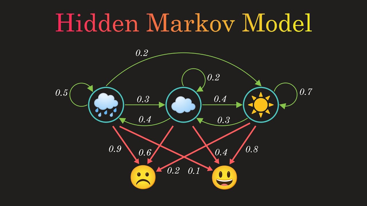
ESE650 begins by developing the probabilistic foundations of algorithms for state estimation, both classical and modern. This includes the properties of joint, marginal, and conditional probability distributions, expectation and covariance of various types of distributions, Bayes Rule, and Markov Chains. We can then use these mathematical tools to develop a generalizable model of markovian systems: the Hidden Markov Model (HMM). This is a powerful and fundamental abstraction used to reason about the observations of the state of a markov chain, where observations are treated as random variables. Mathematically, HMMs are best represented with a transition matrix \( T \) and an emission matrix \( M \). The entry at (i,j) in a transition matrix, \( T_{i,j} \), describes the probability of transitioning from state \( x = i \) to state \( x = j \). The entry at (i,j) in an emission matrix, \( M_{i,j} \), describes the probability of making observation \( y = j \) when the system is in state \( x = i \). The HMM framework allows for concise mathematical formulation of many problems in state estimation, such as filtering, smoothing, prediction, decoding, and observation likelihood.
The first homework in ESE650 introduces students to the above topics by implementing a Bayes Filter, an HMM, and the forward and backward algorithms, Viterbi's Algorithm, and the Baum-Welch Algorithm. This primes students with an understanding of the basics of robot state estimation. An accurate and precise state-estimation system is one of the first steps, if not the first step, to deploying robotic systems into the real world.
With a fundamental understanding of state estimation in-hand, we now examine some of the most popular and useful algorithms for state estimation. A Markov Decision Process (MDP) is a useful formulation for systems where the dynamics or observations cannot be comprehensively or correctly written in the matrix forms for HMMs. In such cases, it is convenient to consider noisy dynamics and observation functional models, i.e. \( x_{k+1} = f(x_{k}, u_{k}) \) and \( y_{k} = g(x_{k}, u_{k}) \). With this formulation, we introduce the Kalman Filter, which is perhaps the most important algorithm in all of robotics. The Kalman Filter works under slightly more specific assumptions than the algorithms we looked at previously. Namely, the basic Kalman Filter is valid under the following conditions:
- Linear Dynamics, i.e. \( x_{k+1} = Ax_{k} + Bu_{k} + \epsilon_{k} \) where:
- \( x \in \mathbb{R}^{d}, u \in \mathbb{R}^{m} \) are the state and control, respectively
- \( A \in \mathbb{R}^{d \times d}, B \in \mathbb{R}^{d \times m} \)
- \( \epsilon \sim \mathcal{N}(0, R), R \in \mathbb{R}^{d \times d} \) is the Gaussian dynamics noise
- Linear Observations, i.e. \( y_{k} = Cx_{k} + Du_{k} + \nu_{k} \) where:
- \( y \in \mathbb{R}^{p} \) is the observation
- \( C \in \mathbb{R}^{p \times d}, D \in \mathbb{R}^{p \times m} \)
- \( \nu \sim \mathcal{N}(0, Q), Q \in \mathbb{R}^{p \times p} \) is the Gaussian observation noise
This essentially constrains the use-cases of the base Kalman Filter to MDPs with linear dynamics models perturbed by gaussian noise, and linear observation models perturbed by gaussian noise. These assumptions are critical in the formulation of the Kalman Gain. Notably, the Kalman Filter is optimal for systems that meet these requirements. However, nonlinear dynamics models and/or the observation models are typical in robotic systems. So how do we handle such cases? Well, we don't; we give up hope and treat the problem as completely intractable and impossible to solve. Obviously, I am joking here; in fact, we have quite a lot of different approaches to solve such problems.
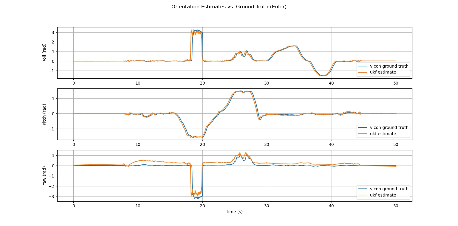
The Kalman Filter can be adapted to cases where the dynamics and/or observations are nonlinear, while keeping the assumption that the noise in these models remains Gaussian. There are several adaptations which exist, but the two KF variants we cover in this course are the Extended Kalman Filter (EKF) and the Unscented Kalman Filter (UKF). The EKF is very straightforward and intuitive, in formulation, application, and explanation. The core principle of the EKF is to use a Taylor Approximation to linearize the dynamics or observations model at timestep \( k \) about the latest filtered estimates. After performing this linearization, the system meets the qualifications of the base KF and as such the KF update equations can be applied without issue. There are cases, however, where the behavior of the linearized system diverges significantly from the behavior of the true system. Such cases are well-handled by the UKF, which leverages the Unscented Transform (UT) to obtain better estimates of system mean and covariance. For the sake of brevity, the UKF uses the UT to construct a set of representative sigma points, and a weighted average is computed to yield mean and covariance estimates of the dynamics and observation models. A more comprehensive understanding of the UKF can be found in chapter 3 of Barfoot et al..
The second homework in this course asks students to formulate and implement an EKF from scratch for an unknown/arbitrary system with nonlinear dynamics and observation models, and similarly implement a UKF for estimating quaternion orientation of a quadrotor from IMU measurements. This assignment gives students the opportunity to learn by experience (and pain) how these algorithms work from the ground up, which is highly beneficial for developing a deep understanding of how modern state-estimation systems work.
We now have a strong understanding of state estimation, whether we like it or not. A natural progression, which this course's curriculum follows, is to examine a class of algorithms called Simultaneous Localization and Mapping (SLAM). SLAM is another critical componnt of the robotics stack. Localization is a special case of state estimation where the state is the robot's pose (position and orientation) and the robot's velocity (oftentimes both linear and angular). Mapping describes the process of capturing perceptual data such as camera images, lidar ranges, and radar data, and combining it with localization information to create a filtering estimate of the surrounding environment. In ESE650, we cover a standard method for probabilistic mapping in two dimensions, which can be extended to three dimensions by leveraging efficient data structures such as kD-trees and octrees. One of my ongoing personal projects is focused on implementing a SLAM stack for an inexpensive quadrotor platform.