Project 1
In MEAM620, Project 1.1 has students create and tune our own nonlinear geometric PD Controller for position and attitude of a quadrotor. In order to properly use a controller, we implement a very primitive trajectory generation routine given waypoints. This subproject generally acquaints students with the simulation environment, nonlinear control, and constant velocity trajectory generation. In Project 1.2, we implement A* Search in 3D, with creative freedom over implementation details and heuristic. My A* Search achieved top-5 performance in the class, where I focused on high efficiency array pre-allocation, intelligent graph representation and traversal, and a well-tuned 3D variant of the Chebyshev/Diagonal Distance Heuristic.
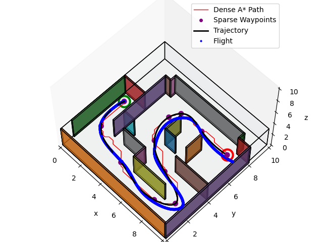
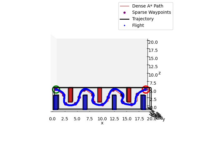
In Project 1.3, we combine these components and iterate upon the full planning and control stack. Our system is given a start pose, goal position, a map with obstacles, and a loose idea of the amount of time it should take to achieve full credit on the assignment. With this, I create an efficient voxelized occupancy grid of the given map and first generate an optimal, dense A* path. Then, I use the Ramer Douglas Peucker Algorithm for pruning the path and generating sparse waypoints. These sparse waypoints are used to first generate a constant velocity trajectory. Then a minimum and maximum speed parameterize a linear interpolation of distance which maps to speed, where longer segments between waypoints have a faster speed. Next, the approximated times of arrival for each waypoint are generated and I use scipy's cubic interpolating spline function to generate 5th order splines between each waypoint, supplying simple boundary condition for the endpoints of the whole path. Now the trajectory is followed as a function of time, where at each timestep of the simulation, the generated trajectory is called and a differentially flat desired state is returned, consisting of position and its first four derivatives (velocity, acceleration, jerk, and snap). The flat outputs are tracked using the same PD controller with better tuned gains. Shown below are some sample results on evaluation maps in a custom simulation environment.
Project 1.4: Bridging the Sim2Real Gap
Part of the MEAM620 curriculum is to explore a very relevant problem in the field of robotics: the sim2real gap. To tackle this problem, students form teams for the only group work in course, and attempt to take the planning and control code written for the simulation in Project 1.3, and deploy it onto a real drone. We wrote up a ICRA-style report to demonstrate our work and findings. Shown below is a video that one of my fine teammates was able to record of our code running on a Bitcraze Crazyflie 2.X drone.
Project 2
In Projects 2.1, 2.2, and 2.3, we step away from the planning and control of quadrotors and instead focus on sensing and perception. Project 2.1 has students implement a complimentary filter to combine accelerometer and gyroscope measurements to estimate the quaternion orientation of the quadrotor. I happened to do this project not long after going through the hell of implementing the Unscented Kalman Filter in ESE650 a few weeks before, so this turned out to be a piece of cake. In Project 2.2, we stepped into the realm of geometric and traditional computer vision by implementing a RANSAC-based pose estimation pipeline for a stereo dataset collected by ETH Zurich. We use an OpenCV ORB-feature extractor and matching routine to rectify the stereo images of the datset, given camera intrinsics. A similar routine is used for performing temporal ORB-feature extraction and matching, to generate approximate visual odometric data. Finally, we implement RANSAC to match these temporal features and provide robust state estimates for the quadrotor pose. Finally, in Project 2.3, we implement Visual Inertial Odometry (VIO) using an Error-State Kalman Filter (ESKF). The ESKF is a variant of Extended Kalman Filter, which tracks the growing error between stereo measurements using IMU data. This improves upon the noisy RANSAC-based state-estimation pipeline created in Project 2.2.
Project 3
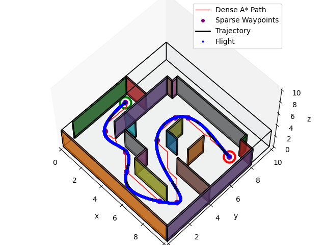
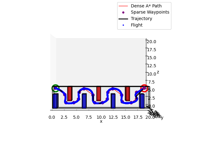
Finally, in Project 3, we create a state-of-the-art (SOTA) software stack for quadrotor navigation in GPS denied environments. We take the optimal planning and control from Project 1.3 and the VIO state estimation module from Project 2.3 to demonstrate a feasible real-world implementation of a semi-autonomous quadrotor. Similar to Project 1.3, it is not enough to simply combine previously written code. Due to much more stringent expectations of speed in navigating the evaluation maps, as well as robustness to simulated sensor noise, we must iterate on our solutions.
I chose to improve upon my existing planning and control modules by implementing a custom minimum-snap optimization routine, drawn from my alma-mater's own Dean of Engineering, Vijay Kumar's seminal work. Additionally, I implemented a minimum-acceleration yaw trajectory generation scheme to help ensure smoother trajectory tracking with uncertainty in our state estimates. With such significant updates to my trajectory generation, I also needed to retune my system's PD controller. With significant tuning of the planning and control modules, I was able to achieve perfect marks on this final project and significantly improved performance as compared to my results from project 1.3. Shown below are sample demonstrations on the same evaluation maps as shown for Project 1.3.